



Image Classification is a computer vision task that aims to assign one or more categories to an entire image based on its visual content. An image goes into the model, and out comes a distribution of scores over the known categories, such as 0.91 for cat, 0.07 for dog, and 0.02 for other.
But building a reliable classification system does not begin with choosing a neural network. The real path is an integrated system that starts before the first line of model code, specifically with the data: collecting it, then cleaning and labeling it, the stage that sets the ceiling on final performance more than any later architectural decision, because label noise and sampling bias flow directly into the model's behavior. Next, the data is split into training, validation, and test sets with a strict separation that prevents information leakage, so the test remains an honest measure of performance the model was never tuned on. Then comes preprocessing and augmentation, which standardize sizes and lighting and generate synthetic variations that curb the model's tendency to memorize training examples.
Only after these preparations is the pretrained model or backbone chosen and put through training or fine-tuning on the task's data. And the work does not end with the first high accuracy: there is an evaluation stage with metrics that respect class balance, then probability calibration and error analysis to expose real failure patterns instead of settling for a single aggregate number. Finally, the system moves into deployment and continuous monitoring, because the production data distribution gradually drifts from the training data, which makes periodic retraining part of the system's design rather than an emergency measure.
Above all of this stands one basic truth:
The model does not "understand" the image the way a human does; it learns numerical representations that help it link visual patterns to specific categories.
Classification and Its Neighbors: Detection, Segmentation, and Face Recognition
Computer vision tasks are often confused with one another, even though each asks a different question and produces a different output:
| Task | The Question It Answers | Output |
|---|---|---|
| Image Classification | What is in the image? | One category for the whole image, such as "cat" |
| Object Detection | What objects are present, and where are they? | A category, Bounding Box, and confidence score per object |
| Image Segmentation | Which pixels belong to which object or region? | A pixel-level mask |
In Object Detection, for example, the model may identify a person, a car, and a traffic light in the same scene and draw a bounding box around each.
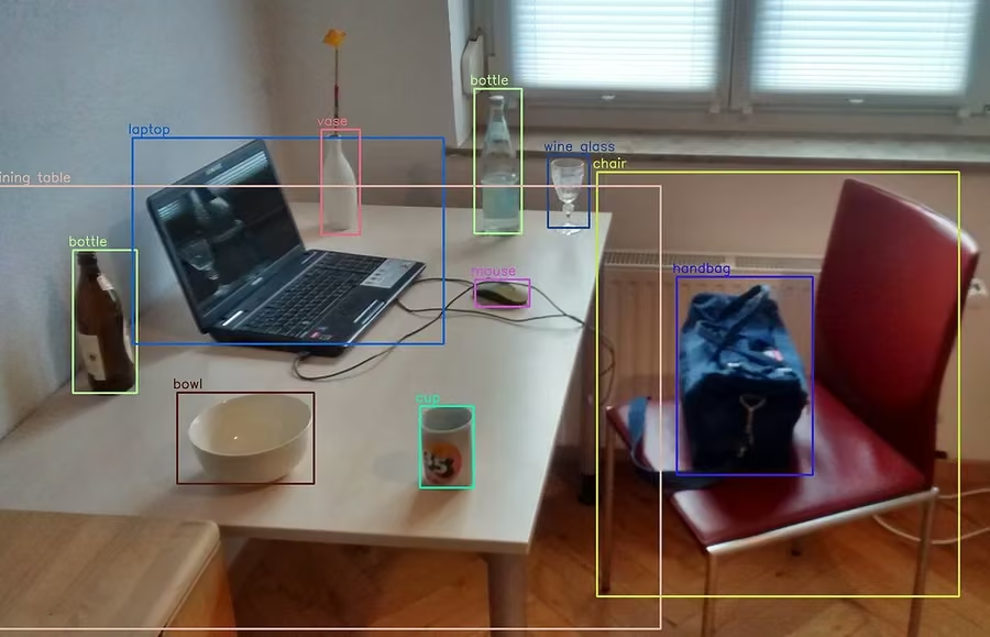
Face Recognition, meanwhile, is not just general image classification; its question is usually "Does this face belong to a specific identity?", it relies on representations and identity matching, and it carries different privacy and security implications. That is why the success of an Image Classifier should not be taken as automatic evidence that an Object Detector or a face recognition system will succeed.
Our AI weapon detection project shows the difference in practice: rather than assigning one label to the whole frame, it uses YOLOv8 to locate a knife or pistol within the camera feed with a bounding box. While building the system we noticed that changes in lighting and in the angles at which objects appear directly affect detection quality, and that balancing processing speed against detection accuracy is an engineering decision made separately for each operating environment.
How Does a Computer See an Image?
To a computer, a digital image is a matrix of values. An RGB image can be represented roughly as height × width × 3 channels, with each pixel holding values for the intensity of red, green, and blue.
Before deep learning, the engineer had to convert these raw values into hand-designed features; today, deep models learn a large part of that representation directly from data. Understanding this shift is the key to understanding the whole history of the field.
From Handcrafted Features to Convolutional Networks
The Classic Pipeline Before Deep Learning
The classic pipeline was staged and manual at its core. It began by extracting hand-designed features through filters and engineering algorithms carefully crafted by researchers, turning raw pixels into a compact feature vector that summarized what was deemed important, such as edges, corners, and textures. That vector was then fed to a traditional classifier that learned the boundaries between classes in feature space. The quality of the entire system hinged on the engineer's skill in designing features; any pattern the descriptor failed to capture was simply lost before it reached the classifier.
Among the best-known feature descriptors are HOG, SIFT, LBP, and Gabor features, and among the classifiers commonly used with them are SVM, Logistic Regression, KNN, and Random Forest.
A Classic Example: HOG + SVM
HOG summarizes the directions of gradients and edges in an image and converts them into a feature vector, after which an SVM learns a boundary separating the classes. This methodology is still useful in some projects, when data is scarce, the problem is relatively simple, compute is limited, the features are well understood, and we need a small, fast model. But it remains more dependent on manual feature engineering.
What Did CNNs Change?
Convolutional Neural Networks — CNNs made it possible to learn features during training itself. Instead of a human designing features and passing them to a classifier, the image now goes straight into a network that learns its own features and then classifies them.
The heart of these networks is the convolutional layer, which applies kernels/filters to local regions of the image. In early layers, responses may emerge to simple patterns such as edges, orientations, contrasts, and textures, and as depth increases the representations become more tied to the structure of objects.
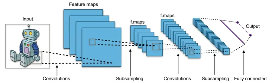
But beware of the popular simplification: "The first layer recognizes edges, the second recognizes eyes, and the third recognizes the face." It is useful for teaching, but it is not a fixed rule for every network and every dataset.
Pooling: Shrinking Spatial Dimensions
Pooling reduces the spatial dimensions of some feature maps, its best-known forms being Max Pooling and Average Pooling.
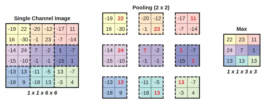
This helps reduce computation, indirectly enlarge the receptive field, and make some representations less sensitive to small local changes. But not all modern networks rely on traditional pooling in the same way; some use strided convolutions or other architectures.
The Classifier Head: Not Necessarily Fully Connected Layers
It is often said that every CNN ends with fully connected layers, which is true of many traditional architectures but not a general rule. Modern models may use Global Average Pooling, a linear classification head, or attention heads. The essential concept, then, is the presence of a Classifier Head that turns the representation into class scores, not the necessity of several fully connected layers.
ResNet: How Deep Training Became Possible
As networks grew deeper, a striking problem emerged: deeper networks do not automatically become easier to train. ResNet introduced the idea of Residual Connections, in which a layer learns the residual and the input is added to it directly:
instead of every layer learning a full transform from scratch. This design helped train very deep networks, and in the original ResNet paper an ensemble of residual networks achieved 3.57% error in the ImageNet 2015 competition.
Precision is needed here:
The 3.57% figure does not mean any single ResNet achieved "96.43% Accuracy" on every kind of image, nor does it mean AI has become better than humans at vision in general.
It is the result of a specific benchmark, within a specific metric, architecture, and experiment.
Beyond CNNs: Transformers and Foundation Models
CNNs remain very powerful, but modern image classification no longer rests on them alone, and the Vision Transformer — ViT was one of the most important shifts.
How Does a Vision Transformer Work?
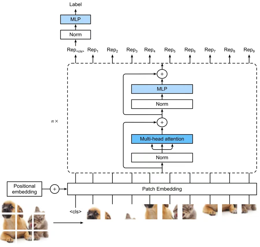
The original ViT idea is conceptually simple: the image is cut into small patches, say 16×16 pixels, and each patch is flattened and passed through a linear projection to become an embedding in the model's processing space, just as a word becomes a token in language models. These embeddings are then treated as a token sequence that flows through the Transformer layers, where self-attention lets each patch "look" at every other patch and decide which ones matter for understanding the whole scene. Finally, the final representation, often via a dedicated classification token, is used to assign the image to its category.
The ViT paper showed that a pure Transformer can achieve very strong image classification performance when pretrained on large data and then transferred to other benchmarks. The landscape thus widened from the conviction that CNNs are the only natural architecture for vision to the recognition that CNNs, Transformers, and others can all learn effective visual representations.
Is a Vision Transformer Always Better than a CNN?
No. The choice depends on data size, the availability of pretraining, resources, latency, the target device, the required accuracy, and model size. A small CNN can be excellent for an edge application, while a ViT or foundation model may win when strong pretraining is available or a broader representation is needed. There is no "best architecture" independent of the use case.
From Closed Sets to Open Vocabularies
Traditional classification is usually closed-set, meaning the classes are known during training, such as cat, dog, horse, and car, and the classifier head learns only those classes. But modern image–text models such as CLIP changed the way of thinking.
CLIP: Classification Through Language
CLIP learns to link images and text within a shared representation space. Instead of a fixed classifier head, an image can be compared with text prompts such as "a photo of a cat," "a photo of a dog," and "a photo of a bicycle," and the closest prompt chosen. This enabled what is called Zero-shot classification on multiple benchmarks without direct supervised training on each dataset.
But that does not mean zero-shot automatically suits every sensitive application; performance depends on the classes, the prompt wording, the domain, the data distribution, and the biases embedded in the pretraining data.
DINOv2: Visual Features Without Labels
DINOv2 is an example of self-supervised visual pretraining, in which the model learns general visual features from many images without relying on traditional labels for each one. That representation can then be used for different tasks, including classification, retrieval, dense prediction, and transfer. This reflects a pivotal trend in computer vision:
Instead of training a separate model from scratch for every project, we increasingly start from a Visual Foundation Model and then adapt it to the task.
Building the Classification Pipeline Step by Step
Having surveyed the architectures, we return to the system sketched in the introduction and build it stage by stage.
Step One: Define the Task Precisely
The first decision is the type of classification: is it Single-label Classification, where each image carries one category, such as cat or dog, or Multi-label Classification, where an image may carry more than one label, such as containing a person, a bicycle, and a helmet at once? The difference is fundamental, because the loss function, the output activation, and the metrics all differ between the two.
Step Two: Collect the Data
Image count alone is not enough. The decisive questions are: Do the images represent the real operating environment? Do they span different cameras, different lighting, and different ages or groups? Do they cover rare cases and diverse backgrounds? And are the labels correct in the first place? A hundred thousand biased images can be worse than a smaller dataset that truly represents the problem.
Step Three: Separate Training, Validation, and Test
The Train set is used to update weights, the Validation set to choose hyperparameters, the checkpoint, the threshold, and the model itself, and the Test set for final evaluation alone.
One of the most dangerous mistakes here is Data Leakage. In medical imaging, for example, if multiple images of the same patient are spread across training and test, performance may look much higher than it really is. The correct split may therefore be at the level of the patient, device, site, or time period, depending on the task.
Step Four: Preprocessing
Preprocessing may include resizing, cropping, normalization, color conversion, and artifact removal. There is no single normalization that is right for everyone; if you use a pretrained model, you most likely need to respect the preprocessing it was trained with.
Step Five: Data Augmentation
Data augmentation may include random cropping, rotation, flipping, color jitter, blur, random erasing, and MixUp/CutMix in some projects. Its goal is not merely to "increase the number of images," but to expose the model to plausible variations it may encounter at runtime.
Augmentation becomes dangerous when it changes a label's meaning: horizontally flipping an X-ray or an image of an organ may change the anatomical side (laterality), and large rotations may be unrealistic for documents or specific orientations. The rule here:
Augmentation must preserve the meaning of the class, not be random just to increase data.
Step Six: Choose a Baseline
Start with something simple: Logistic Regression on ready-made features, an SVM, a pretrained ResNet18, a MobileNet/EfficientNet-class model, or a small ViT. The goal is to find out whether any added complexity brings real value.
Step Seven: Transfer or Train from Scratch?
In many projects, Transfer Learning is the practical choice, and it has two common styles. The first is the Fixed Feature Extractor, freezing most of the backbone and training only the classification head. The second is Fine-tuning, starting from pretrained weights and then updating some or all of the model's layers.
So transfer does not always mean "freeze the early layers and train only the last layer"; that is one method among several. Full fine-tuning may be better when there is enough data, the domain is different, and a suitable learning rate is used.
Step Eight: Understand What the Model Outputs
A multi-class classifier usually produces raw values called logits, such as [4.2, 1.1, -0.4], which a Softmax function then turns into values summing to 1, such as [0.94, 0.043, 0.017]. But there is an important caveat:
A Softmax score is not necessarily a well-calibrated probability.
The model may be overconfident, which is why high-stakes applications need calibration instead of interpreting 0.94 as true 94% confidence.
How Do We Measure a Classifier's Performance?
Overall Accuracy and Its Trap
Accuracy is defined as follows:
It suits cases where classes are relatively balanced and error costs are similar, but it can be misleading. Take a dataset with 990 healthy images and 10 diseased images: a model that says "healthy" for every image achieves 99% accuracy, yet its Recall for the diseased cases is 0%, meaning it fails the medical goal completely.
Precision, Recall, and F1
Precision answers the question: of everything the model predicted as positive, how much was correct?
Recall answers the question: of the truly positive cases, how many did the model find?
The F1 Score is the harmonic mean of the two, useful when we need a balance between them:
Macro or Weighted F1?
In multi-class classification, Macro F1 computes F1 for each class and then gives them all equal weight, which is useful when rare classes matter. Weighted F1 weighs each class by its number of samples, and may thereby hide poor performance on a small class.
The Confusion Matrix
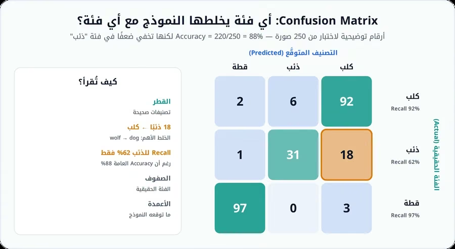
The Confusion Matrix is one of the most valuable tools, because it reveals which class the model confuses with which. We may discover that it confuses wolves with dogs, trucks with buses, and melanoma with a benign lesion, and this information matters far more than a single accuracy figure.
ROC-AUC and PR-AUC
These metrics can be useful especially in binary classification, but the choice of metric should rest on class imbalance, the cost of false positives, the cost of false negatives, the threshold, and the nature of the application. On highly imbalanced data, a Precision-Recall curve may be more informative than accuracy alone.
From the Dataset to the Real World
Distribution Shift
Success on the test set is not enough, because of the problem of Distribution Shift. A model may train on images from professional cameras and then run on a cheap phone, train on data from one hospital and then be used in another, or train in good lighting and then operate at night. It must therefore be tested on different devices, locations, and times, under blur, lighting changes, compression, and occlusion, and on the subgroups that matter.
Confidence Is Not Certainty
A model may output 0.99 for dog while the image lies entirely outside the training distribution: an X-ray in front of a model trained on animals, an odd cartoon drawing, or a type of disease it has never seen. Good systems therefore sometimes need out-of-distribution detection, abstention, human review, confidence thresholds, and calibration. The best decision may be "I don't know enough" rather than a wrong class with high confidence.
Deep Learning or Classic Machine Learning?
Academic sources often contrast the two approaches sharply, but reality depends more on the task:
| Classic ML Is Preferable When | Deep Learning Usually Wins When |
|---|---|
| The dataset is very small | The visual data is complex |
| The features are well understood and strong | Pretrained models are available |
| Resources are limited | We need to learn features |
| The model needs to be simple | Visual variation is high |
| Latency must be extremely low | The scale is large |
| We need a relatively direct explanation |
Most importantly, Transfer Learning has greatly narrowed the gap in data requirements. The claim that deep learning always needs millions of images was truer when thinking centered on training from scratch; today you can start from a pretrained ResNet or ViT, a self-supervised model, or an image–text model, and then fine-tune on a smaller dataset. But "smaller" does not mean any number of images will do; quality, representativeness, and similarity to the original domain remain decisive.
Applications of Image Classification
Medical Imaging
Models may assist in reading mammograms, retinal images, skin lesions, pathology slides, X-rays, MRI, and CT. But research performance must be kept separate from clinical deployment.
A 2020 Nature study on breast cancer screening showed, on the study's dataset, an absolute reduction in false positives of 5.7% in the United States and 1.2% in the United Kingdom, and a reduction in false negatives of 9.4% and 2.7% respectively. These are the results of a specific study, not a statement that "AI is more accurate than doctors at every diagnosis," and an addendum was later published to add detail on the method's reproducibility. That is why any medical system needs external validation, clinical validation, regulatory review where applicable, continuous monitoring, and human oversight.
Vehicles and Autonomous Driving
Computer vision matters for vehicles, but Image Classification alone is not enough; a vehicle usually needs object detection, segmentation, tracking, depth estimation, sensor fusion, planning, and control.
The popular phrase "94% of crashes are caused by human error" must also be handled with care. NHTSA documents clarify that the "Critical Reason" is the last failure in the chain before the crash, and is neither the cause of the crash nor an assignment of fault. So it is not valid to turn such a figure into a claim that machine vision systems will automatically prevent 94% of crashes.
Manufacturing
Classification is used for defect classification, product quality control, sorting, part-type identification, and surface-condition monitoring. In its simplest form, a camera captures an image of the part on the production line and the model classifies it directly into one of the defined categories: intact, scratched, cracked, or surface-contaminated, with the verdict based on a confidence threshold set by the production plan. This is enough when the question is "Is the part acceptable?", but if the facility needs to determine where the defect is and its boundaries on the surface, classification becomes the wrong tool, and moving to Detection or Segmentation is the better solution.
Agriculture
In agriculture, classification is used to identify plant diseases, crop types, fruit ripeness, and produce quality, but the model must be tested on different cameras, under sunlight, in different environments, and on diverse plant varieties.
Security and Surveillance
Classification can be used here to categorize scenes, content, and visual events. Face Recognition, however, is a different and sensitive task, in which false matches, performance across demographic groups, consent or legal basis, data retention, and security must all be assessed. A model with high accuracy on a public dataset should not be taken as evidence of its suitability for a high-risk identity use.
Challenges, Robustness, and Interpretability
Data and Learning Challenges
Classification systems fail for many reasons, summarized in the table below:
| Challenge | What Happens |
|---|---|
| Label Quality | If labels are wrong, the model learns noise |
| Class Imbalance | The model may ignore rare classes |
| Shortcut Learning | It learns an unintended signal, such as a device mark, a background, or a marker on an X-ray instead of the disease itself, then collapses outside the dataset |
| Domain Shift | A change in camera, location, or population can lower performance |
| Spurious Correlations | The label may correlate with a side factor only in the training data |
Adversarial Examples
Research has shown that specially designed perturbations can push models into wrong classifications with high confidence. But adversarial attacks are not just "invisible noise"; there are also physical adversarial patterns, patch attacks, and data poisoning, and defending against all of them is not a fully solved problem.
Adversarial Training can increase robustness against certain families of attacks, but it may raise training cost, affect accuracy on clean data, and fail to generalize to every threat model. So choosing a defense must be preceded by a clear question:
Who is the attacker? What can they do? And what do we want to protect?
How Do We Understand the Model's Decision?
Tools such as Grad-CAM can produce an approximate heatmap of the regions that contributed to a prediction within some CNN-based architectures. This is useful for debugging, detecting shortcut learning, and reviewing what the model actually looks at. But:
A heatmap is not a complete causal explanation, nor proof that the model "thought" this way like a human.
The explainability tool itself needs evaluation.
Deploying on Edge Devices
We may need to run classification on a phone, a camera, a Raspberry Pi-class device, or an embedded accelerator. Several tools serve this purpose, summarized in the table below:
| Technique | The Idea |
|---|---|
| Quantization | Reducing numerical precision, such as moving from FP32 to INT8 |
| Pruning | Removing some low-importance weights or structures according to a defined method |
| Knowledge Distillation | Training a smaller student model to benefit from a larger teacher |
| Smaller Backbone | Sometimes the best optimization is choosing a smaller model from the start |
Whatever the tool, you must measure accuracy, latency, RAM, model size, power consumption, and throughput, not FLOPs alone.
How Are Foundation Models Changing the Future of Classification?
The field is shifting from a model trained only for fixed classes to a general visual representation that can be adapted to many tasks. CLIP links images and text and enables zero-shot classification in many cases, DINOv2 learns general visual features in a self-supervised way, and ViT-based pretrained models can be fine-tuned or have their features used directly.
These models reduce the need for training from scratch, but they do not remove the need for local validation, bias testing, data governance, and domain testing.
How Do You Choose an Approach in Practice?
The simplified decision below links the nature of a project to the right starting point:
| Project Situation | Where to Start |
|---|---|
| Small dataset and a clear task | A pretrained CNN or ViT with Transfer Learning |
| A small edge device | A mobile-oriented CNN, a small ViT, or a quantized model |
| Constantly changing classes | Image-text models, embedding-based classification, or a retrieval-assisted approach |
| A sensitive medical or industrial domain | Dataset quality, external validation, calibration, error analysis, human review, and monitoring |
| Not enough labels | Self-supervised pretraining, Transfer Learning, Active Learning, weak supervision, or vision-language models |
A Checklist Before Launching a Classifier
Before a classifier reaches production, the following points should be confirmed, distributed across the stages of the system:
| Stage | What to Verify |
|---|---|
| Task definition | The task is truly Classification, not Detection/Segmentation, and the classes are clearly defined |
| Data | Labels reviewed by specialists where needed, Train/Val/Test sets separated without leakage, and the test set represents the real world |
| Modeling | A baseline exists, and class imbalance has been handled appropriately |
| Evaluation | Metrics chosen according to the cost of error, the confusion matrix reviewed, and subgroup evaluation in place where needed |
| Reliability | The model is calibrated if scores will be used as probabilities, its out-of-distribution behavior is known, and a human fallback exists for critical decisions |
| Operations | Latency, power, and memory tested on the real device, post-deployment monitoring in place, and a retraining and versioning plan ready |
Conclusion
Image classification no longer means an image going into a CNN and a label coming out. The modern system is an integrated whole built by accumulation rather than in a single step: it starts with representative data reflecting the real distribution the system will face, passes through preprocessing and augmentation that broaden training coverage, and then draws on a pretrained visual representation inside a CNN, ViT, or foundation model instead of learning everything from scratch. Then comes fine-tuning on the task's data, producing probability scores rather than rigid labels, which in turn undergo calibration, metrics, and error analysis that expose weaknesses before the user does. And at deployment the story does not end, as continuous monitoring tracks data drift and performance degradation and feeds an improvement loop that returns to the data once more.
Historically, the field has traveled a long road: it began with hand-crafted features extracted by methods such as SIFT and HOG and fed to a classifier such as an SVM, then convolutional neural networks (CNNs) arrived to learn these features from the data itself, followed by deeper networks such as ResNet, then the Vision Transformer, which reduced the need for large volumes of labeled data through pretraining, until today we have reached self-supervised and multimodal vision-language foundation models. But the newest model is not automatically the best.
The best system is the one that solves the right task, trains on representative data, is measured with metrics suited to the risks, knows when not to trust its prediction, operates within resource limits, and proves its performance in the environment where it will actually be used.
Sources and References
K. He et al. — Deep Residual Learning for Image Recognition
https://arxiv.org/abs/1512.03385A. Dosovitskiy et al. — An Image is Worth 16×16 Words: Transformers for Image Recognition at Scale
https://arxiv.org/abs/2010.11929OpenAI — CLIP: Connecting Text and Images
https://openai.com/index/clip/M. Oquab et al. — DINOv2: Learning Robust Visual Features without Supervision
https://arxiv.org/abs/2304.07193PyTorch — Transfer Learning for Computer Vision Tutorial
https://docs.pytorch.org/tutorials/beginner/transfer_learning_tutorialscikit-learn — Metrics and scoring: quantifying the quality of predictions
https://scikit-learn.org/stable/modules/model_evaluation.htmlS. M. McKinney et al. — International evaluation of an AI system for breast cancer screening
https://www.nature.com/articles/s41586-019-1799-6McKinney et al. — Addendum: International evaluation of an AI system for breast cancer screening
https://www.nature.com/articles/s41586-020-2679-9R. R. Selvaraju et al. — Grad-CAM
https://arxiv.org/abs/1610.02391I. Goodfellow, J. Shlens, C. Szegedy — Explaining and Harnessing Adversarial Examples
https://arxiv.org/abs/1412.6572NHTSA — Critical reason is not the cause of a crash / crash causation guidance
https://www.nhtsa.gov/sites/nhtsa.dot.gov/files/812023-heavy_truck_pre-crash_scenarios.pdfO. Russakovsky et al. — ImageNet Large Scale Visual Recognition Challenge
https://arxiv.org/abs/1409.0575C. Shorten, T. M. Khoshgoftaar — A survey on Image Data Augmentation for Deep Learning
https://journalofbigdata.springeropen.com/articles/10.1186/s40537-019-0197-0
Official documentation & standards
Frequently Asked Questions
What is AI image classification?
It is training a model to assign one or more classes to an entire image based on the patterns it learned from previous data.
What is the difference between image classification and object detection?
Classification assigns a class to the image, while object detection also localizes objects within it using bounding boxes or an equivalent representation.
Are CNNs still used?
Yes. CNNs remain highly effective, especially in practical and edge applications, but they are no longer the only architecture; Vision Transformers and foundation models have also become important.
What is a Vision Transformer?
A model that splits the image into patches and treats them as a sequence of tokens passed through a Transformer to extract a representation for classification or other visual tasks.
Must the model be trained from scratch?
Usually not. Transfer learning or fine-tuning a pretrained model is often a very practical choice.
Is accuracy enough to evaluate a model?
No, especially with class imbalance. You should also look at precision, recall, F1, the confusion matrix, and metrics that match the cost of errors.
What is the difference between precision and recall?
Precision measures how many positive predictions were correct, while recall measures how many real positive cases the model managed to detect.
Does a 90% softmax score mean the model is 90% certain?
Not necessarily. Scores may be uncalibrated and the model may be overconfident; calibration can be used when needed.
What is zero-shot image classification?
Classifying classes the model was never directly trained on in the traditional supervised sense, for example using an image-text model to compare the image against descriptions of the classes.
What is CLIP?
A model that learns joint representations of images and text and can be used for zero-shot classification and other tasks that rely on similarity between an image and a description.
Technical Discussion (0)
Sign in to join the discussion, reply and like comments.


