



Smart ride-pooling (Dynamic Ride-Pooling) is an on-demand transport system that tries to combine passengers with compatible routes in the same vehicle in real time, while balancing competing goals: reducing passenger waiting, reducing each passenger's detour, raising vehicle occupancy, cutting empty distance, and improving fleet efficiency.
The idea looks simple: one passenger sets off from X heading to Y, and another sets off from a nearby point toward a nearby destination, so they share the same vehicle and a single trip serves two requests instead of two. This combining is the core of the system's economic and environmental value, and at the same time the source of its complexity: every additional passenger means extra deviations from the optimal route and a longer wait, turning "picking up a companion along the way" into a delicate equation that balances each passenger's comfort against fleet efficiency.
But carrying out the idea across an entire city is far from "finding the nearest car." The real system solves a problem that changes every second: new requests arrive constantly, vehicles are moving, passengers are already on board some vehicles, travel times shift with traffic, each passenger has an acceptable limit for waiting and detour, capacity is limited, some requests cannot be combined without harming service quality, and every decision made now affects where a vehicle will be in a few minutes and its ability to serve the next request.
That is why a modern ride-pooling system is closer to a real-time optimization platform that never stops: it takes requests, vehicle positions, traffic conditions, and operational constraints as inputs refreshed every second, feeds them into a matching and routing engine that generates shared trips and fleet rebalancing decisions, and recalculates everything whenever the state changes, which happens constantly. The system does not "solve" the problem once; it lives in a perpetual cycle of re-optimization.
Ride-Hailing and Ride-Pooling: A Fundamental Difference
The two terms are sometimes used as if they were the same thing, but the difference between them is decisive. In Ride-Hailing, a digital platform connects a single passenger or group with a driver or vehicle, like a private trip through an app: passenger A in vehicle 1, passenger B in vehicle 2, and passenger C in vehicle 3.
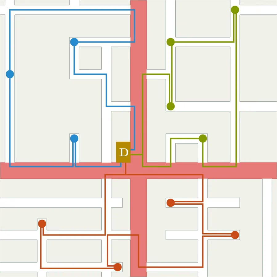
In Ride-Pooling, the platform tries to combine independent requests in the same vehicle if they are compatible. Passengers A, B, and C each have a different origin and destination, but the matching engine checks whether their routes intersect within an acceptable detour range, and assigns all three to a single vehicle that serves them in one ordered tour instead of three separate ones. Compatibility here is not just geographic proximity; it includes allowed pickup and drop-off times and vehicle capacity, the constraints that separate a successful combination from a poor service experience.
The FHWA describes ride-sharing in the on-demand transport context as a situation in which passengers choose a product that allows their trips to be matched with other passengers who have overlapping routes.
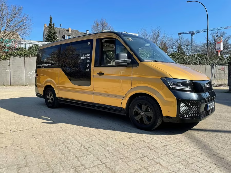
The takeaway:
All Ride-Pooling is on-demand transport, but not all Ride-Hailing is actual ride sharing.
This difference is fundamental when the conversation turns to congestion and emissions.
Do Ride-Hailing Apps Reduce Congestion Automatically?
No. The idea may seem logical: if people use a car they do not own, there will be fewer cars. But the system can add new kilometers through cars driving without passengers between requests, heading to pickup points, drawing in people who would otherwise have taken the bus, metro, or walked, and generating new trips that would never have happened at all. The distance a vehicle travels without passengers is called Deadheading.
In a study of about 1.5 million RideAustin trips, drivers' travel to and from the service area was estimated at 19% of the service's total vehicle miles traveled (VMT), while driving between trips made up another 26% by the study's estimate. These are figures from a specific case study, not a fixed global percentage. A study published in Science Advances also found that the spread of transportation network companies in San Francisco contributed to increased congestion during the studied period from 2010 to 2016.
Therefore:
App-based transport is not synonymous with sustainable shared transport.
The real question is:
Does the system raise average occupancy and reduce Vehicle Kilometers Traveled after accounting for empty distance, detours, and changes from the original travel mode?
When Can Ride-Pooling Reduce the Number of Vehicles?
The benefit materializes when the system succeeds in combining requests that would otherwise have needed separate vehicles. Take three passengers, A, B, and C, each of whom would need a private vehicle in the traditional scenario, traveling 8, 7, and 9 kilometers respectively, for a total of 24 vehicle-kilometers. If all three are combined into a single vehicle that travels only 13 kilometers, total vehicle kilometers traveled (VKT) falls by roughly half.
But if the pickup points are far apart, so that the detour reaches:
the benefit may vanish entirely. Success depends on demand density, the similarity of origins and destinations, the waiting window, the acceptable detour limit, fleet size, vehicle capacity, request timing, and matching quality.
Why Is Dynamic Pooling a Hard Problem?
Suppose there are 5,000 vehicles, 20,000 active requests, and several passengers inside some vehicles. It is then impossible to test every possible combination naively, because each new request might be inserted before another passenger's pickup, after it, between drop-offs, or be rejected. And in every case the following constraints must be respected:
| Constraint | Meaning |
|---|---|
| vehicle_capacity | The vehicle's capacity |
| maximum_wait_time | The maximum waiting time |
| maximum_detour | The maximum deviation from the route |
| pickup_time_window | The pickup time window |
| dropoff_time_window | The drop-off time window |
| driver_constraints | Driver constraints |
| service_area | The service area |
The problem is therefore tied to well-known families of problems, such as Dynamic Vehicle Routing, the Dial-a-Ride Problem, Assignment, and Combinatorial Optimization, problems that can become extremely hard computationally as their size grows.
The Complete Path of a Passenger Request
A request's journey through the system passes through a series of stages, each with a different goal. The passenger request enters and is first validated: sound coordinates, a covered area, and complete data. Then the fleet is searched for nearby available candidate vehicles, on top of which the engine generates the feasible shared trips that satisfy every constraint, estimating the pickup time and detour size for each option; the alternatives are then evaluated with an objective function that balances passenger satisfaction against fleet efficiency, before the vehicle is assigned and its route updated. After execution, the system keeps tracking the trip moment by moment, and when the state changes, through a new request, sudden congestion, or a cancellation, the calculations are redone. No decision is made once and finished; the trip remains a living entity whose plan is continually revised.
Receiving the Request
A typical request may contain the pickup location (pickup_location), the drop-off location (dropoff_location), the request time (request_time), the maximum acceptable wait (max_wait), the maximum acceptable detour (max_detour), the number of passengers (passenger_count), and accessibility needs. The system should not collect additional data it does not need.
Searching for Candidate Vehicles
Instead of comparing the request with every vehicle in the city, the search can be narrowed by estimated time of arrival (ETA) to the pickup point, geographic area, available capacity, current trip direction, and whether the request can be inserted into the existing route. This step shrinks the search space dramatically.
Can a New Passenger Be Inserted into an Existing Trip?
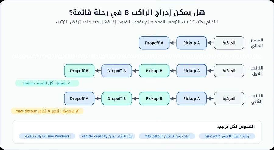
Suppose a vehicle's current route serves passenger A alone: pick them up, then drop them off. When a new request arrives from passenger B, there is no single correct way to insert it; the system might try picking up B before A and dropping B off afterward, or picking them up together and dropping B off first if B's destination is closer. For every possibility, the system recalculates: How much will B's wait increase? How much will A's trip time increase? Is capacity exceeded? Are the time windows still valid? If any constraint fails, the request cannot be inserted into this vehicle.
The Request-Trip-Vehicle Graph
One of the best-known and most influential research frameworks in dynamic ride-sharing is the work of Alonso-Mora and colleagues, published in 2017, which solves the problem through four stacked layers: it first determines which requests can be shared at all, then builds the feasible shared trips that meet the time and space constraints, then computes the compatibility of each trip with each vehicle as a system of acceptable pairs, and finally solves the global assignment that distributes trips among vehicles at the best overall value. Together, these four layers are what turn a chaotic list of requests into a single coherent operating plan.
In the study's experiment on data from about 3 million New York taxi trips, the researchers showed that a dynamic matching algorithm built on this framework could achieve high service rates with a smaller fleet in the simulation model, with a clear trade-off among fleet size, vehicle capacity, waiting time, and passenger delay. But these are simulation results on a specific dataset and scenario, not a promise that any city will get the same percentages.
Why Not Just Use Greedy Matching?
Greedy matching says: give the request to the nearest vehicle available right now. It is fast, simple, and easy to operate, but it may produce a bad decision five minutes later. Vehicle A may be closest to a small request, while a minute later two highly compatible requests appear in A's own area; if A is used now, a better pooling opportunity may be lost later. This is the difference between a myopic decision and an anticipatory decision.
The Algorithms Used in Ride-Pooling
No single algorithm suits every platform; instead there are families of methods, each with its place:
| Family | The Idea | When It Fits and Its Limits |
|---|---|---|
| Greedy / Insertion Heuristics | Testing the insertion of a new request into an existing route | When we want speed, a strong baseline, and a simpler system |
| Integer / Mixed Integer Optimization | Formulating assignment as an optimization problem | When we need a better overall solution and clear constraints, though compute time can become a challenge at large scale |
| Metaheuristics | Such as Large Neighborhood Search, Genetic Algorithms, and Simulated Annealing | They may find good solutions in large search spaces, with no guarantee of being faster or better in every scenario |
| Machine Learning | Used in parts of the system rather than replacing optimization entirely | ETA estimation, demand forecasting, acceptance probability, travel time, and candidate pruning |
| Reinforcement Learning | Learning policies for long-horizon decisions | Rebalancing, pricing, zone selection, and anticipatory control, but it is no magic solution for the matching problem |
In many of the strongest research systems, the design is hybrid: machine learning predicts, optimization decides, and simulation evaluates. Or the work is split between two layers: a GNN or RL model chooses the strategic action, such as which zone to replenish with vehicles and which matching policy to activate, while the assignment solver enforces the hard constraints without compromise: the vehicle must not exceed its capacity, and no passenger's pickup time may be violated. With this division, the system benefits from learned intuition without handing it a decision that breaks a non-negotiable operational constraint.
Why Use Graph Neural Networks (GNNs)?
A road network is a graph by nature: each zone or intersection is a node, and each road connecting them is an edge. This structure has a key advantage: high demand in one zone spills over within minutes into neighboring zones, which graph models capture better than models that treat each zone as an isolated unit. A GNN can build a representation of the state that combines each zone's demand, the number of vehicles available in it, travel times, and congestion in neighboring zones, and then produce embeddings representing the spatial relationships among these elements.
In practice, the whole city is built as an urban graph whose network passes through the GNN to produce a spatial representation capturing the relationships between zones, and this representation in turn feeds the reinforcement learning, prediction, or optimization layers that make the actual decision. The GNN here is not a decision-maker but a producer of spatial understanding: it turns a scattered map of numbers into a connected picture on which the rest of the system builds.
But using a GNN does not automatically mean the model beats traditional methods; it must be compared with baselines under the same data, the same constraints, the same compute budget, and the same KPIs.
What Is the Role of Deep Reinforcement Learning?
In ride-pooling, the current decision affects the future. Sending a vehicle to the west side of the city now may yield a lower immediate reward, but high demand density may appear there ten minutes later. That is why reinforcement learning tries to learn a policy that maximizes reward over an extended time horizon rather than for a single decision. Its formulation has three elements:
| Element | Its Content in Ride-Pooling |
|---|---|
| State | The distribution of vehicles across zones, active requests, expected demand over the coming minutes, traffic conditions, and seat occupancy in each vehicle |
| Action | Repositioning a vehicle toward another zone, changing its operating zone, prioritizing a group of requests, or adjusting a parameter in the policy itself |
| Reward | Combines what should be maximized, such as served trips and occupancy, with what should be minimized: waiting time, detour, empty driving, rejected requests, and an emissions indicator |
But reward design is extremely sensitive: if a large weight is given to revenue alone, the system may ignore fairness, and if a large weight is given to occupancy, it may impose annoying detours.
Is MADRL-GNN the Ideal Architecture?
The original research thread proposes combining Multi-Agent Deep Reinforcement Learning + Graph Neural Networks, a logical idea from a research standpoint, because there are many vehicles, the network is a graph, decisions are sequential, and demand varies in space and time. But this should not be turned into the claim that:
MADRL-GNN is the best proven algorithm for ride-pooling.
A fair comparison requires a complete implementation, baselines, hyperparameter tuning, multiple random seeds, real datasets, ablation studies, statistical significance, accounting for compute cost, and out-of-distribution tests.
Nor is the claim that inference becomes O(1) after training generally true; the cost of a GNN depends on the number of nodes, edges, layers, and feature size, and the cost of the assignment solver depends on the number of vehicles, requests, feasible trips, and constraints.
Fleet Rebalancing
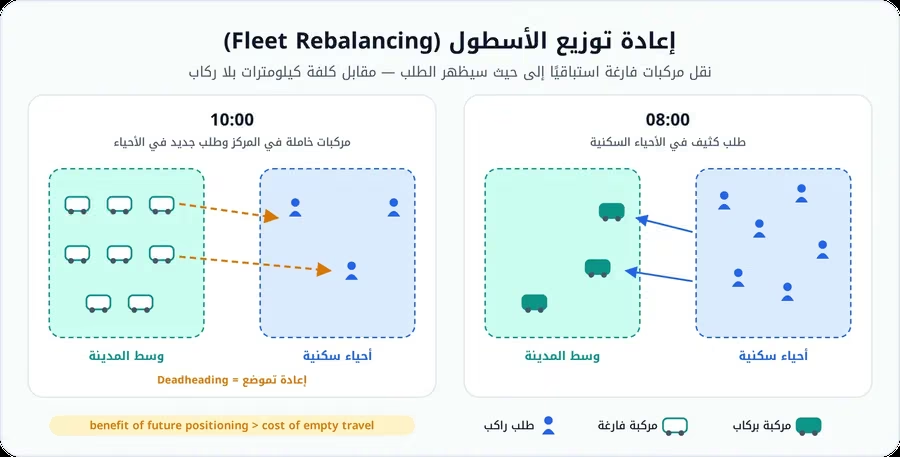
Even if matching is excellent, the fleet may cluster in the wrong place. At 8 a.m., requests pour in from residential neighborhoods, so vehicles carry their passengers downtown, leaving few vehicles in the neighborhoods later. By 10 a.m., empty vehicles pile up downtown while new demand appears in the neighborhoods. This is where rebalancing comes in: proactively directing empty vehicles toward where demand will appear.
But there is a paradox here:
Repositioning helps reduce waiting, but it adds Deadheading.
So the benefit of future positioning must outweigh the cost of traveling empty.
How Do We Predict Demand?
Inputs and Models
Demand Forecasting tries to estimate the number of requests in each zone at each time, based on historical demand, time of day, day of week, weather, events, holidays, public transit disruptions, and the current demand trend. Time-series models, gradient boosting, LSTM/GRU, Temporal CNNs, GNNs, and Transformers can all be used. But there is no single "gold standard"; the best model depends on the dataset, spatial granularity, forecast horizon, and the city's dynamics.
Is a 15–45-Minute Horizon Always Appropriate?
No. The forecast horizon must be chosen according to the operational decision it serves:
| Forecast Horizon | The Decision It Serves |
|---|---|
| 5 minutes | Near-term rebalancing |
| 30 minutes | Fleet positioning |
| Hours | Staffing, charging, and supply planning |
What matters most is not forecast accuracy alone; a less accurate model may drive better fleet decisions. That is why the operational value of the forecast must be measured, not RMSE alone.
The Architecture of a Real Ride-Pooling Platform
The Real-Time Path and the Non-Real-Time Path
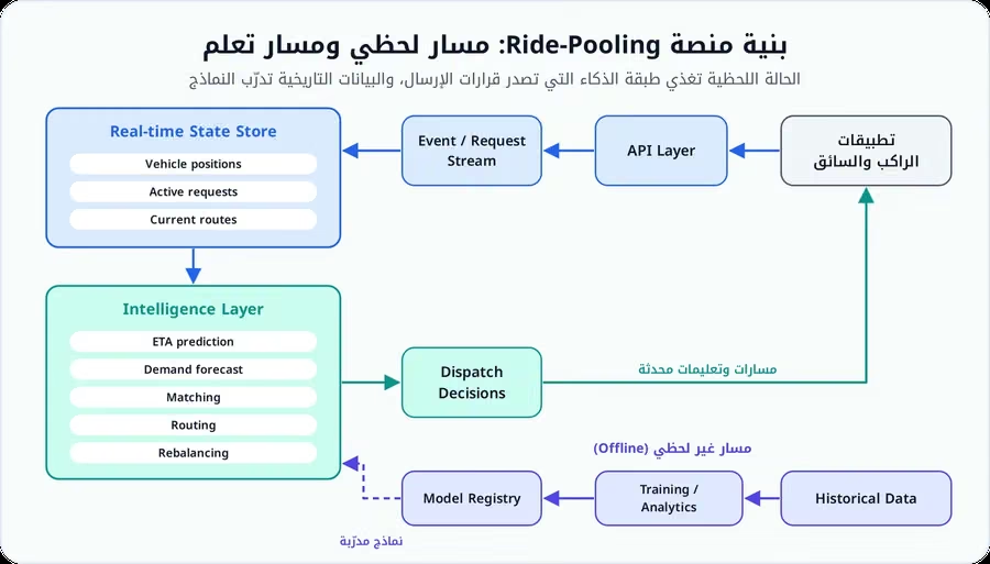
The platform is designed in layers starting from both ends of the experience: the passenger and driver apps connect to an API layer that captures requests and location updates, all of which flows through a never-ending stream of events and requests and accumulates in a real-time state store that keeps a live snapshot of the system: the positions of all vehicles, active requests, and routes in progress. On top of this store runs the intelligence layer, which produces ETA and demand predictions and handles matching, routing, and rebalancing, issuing dispatch decisions that return to the driver and passenger apps to be executed on the road. The cycle thus completes from app to app, with each link consuming the output of the one before it.
Alongside this real-time path runs a parallel non-real-time path: historical data accumulates to feed training and analytics, and the resulting models are stored in a model registry that manages their versions and deployment to production. Separating the two paths is deliberate; the real-time system must respond in fractions of a second, while improvement from yesterday's data proceeds at the rhythm of days, and each path has an entirely different infrastructure.
Do We Really Need Big Data?
Not every system needs "Big Data." A small platform in a limited city may run efficiently with a geographic database, simple stream processing, and an optimization service. The term Big Data becomes meaningful when volume, velocity, or variety reach a level that genuinely requires a distributed architecture. The goal is not "using Kafka and a Data Lake because the system is smart," but building the simplest architecture that can meet the required service-level agreement (SLA).
What Data Does the System Need?
| Source | Data |
|---|---|
| The passenger | Origin, destination, request time, party size, maximum waiting preference, and accessibility needs where relevant |
| The vehicle | Current location, route, occupied seats, capacity, status, and energy or fuel level if it matters |
| The network | Travel times, closures, incidents, and congestion |
| Historical data | Demand by zone and time, cancellations, wait times, pickup success, detours, and deadheading |
Map Matching
GPS does not always give an accurate position on the road; a point may appear ten meters beside it. That is why map matching links telemetry to the nearest logical segment of the road network, an important step because route optimization depends on a correct graph.
Is Edge Computing Necessary?
Not always. Many ride-pooling systems run in the cloud or in data centers, because dispatch decisions are centralized by nature. Edge computing may help with local traffic processing, filtering data to protect privacy, connected vehicle systems, and low-latency roadside analytics. But putting "AI inside every vehicle" is not a prerequisite for dynamic pooling.
How Do We Define the Objective Function?
A poorly designed system may achieve one metric while harming the rest. Minimizing distance traveled alone may lengthen passengers' waits, minimizing waiting alone may dispatch many separate vehicles, and maximizing occupancy alone may impose large detours. That is why we need multi-objective optimization, a simplified example of which is:
The weights here are not "fixed scientific values"; they express policies and business goals, and the sensitivity of results to them must be tested.
The Right Performance Indicators
Five Families of Indicators
| Family | Indicators |
|---|---|
| Passenger experience | Mean wait, P90/P95 wait, in-vehicle time, detour time, cancellation rate, rejection rate, and pickup reliability |
| Fleet | Vehicle occupancy, pooling rate, deadheading distance, revenue kilometers, idle time, and trips per vehicle-hour |
| Network | Total VKT, VHT, average speed, and congestion delay |
| Sustainability | Fuel or energy use, CO₂e, and emissions per passenger-km |
| Fairness | Wait time by zone, rejection by zone, service coverage, and accessibility |
Fairness indicators in particular are what prevent the system from improving only downtown while leaving the outskirts with poor service.
Why P95 Sometimes Matters More Than the Mean
An average wait of 4 minutes may look excellent, but if 10% of users wait 18 minutes or more, there is a real problem. So monitor the whole distribution, not just the mean.
How Do We Measure Congestion?
Counting the vehicles we saved in theory is not enough. Vehicle Kilometers Traveled (VKT), Vehicle Hours Traveled (VHT), Vehicle Hours of Delay (VHD), speed, queue length, and network throughput must be used. And the calculation must include every kind of travel: occupied travel, empty driving toward pickups, empty driving between trips, rebalancing, and detours.
Emissions: The Full Picture
Does Ride-Pooling Always Reduce Emissions?
No. The environmental benefit is the outcome of an equation: avoided vehicle travel, minus new deadheading, pooling detours, and the effect of mode substitution. If a person switches from a private car to a shared ride, a benefit may appear. But if they switch to it from the metro, the bus, walking, or cycling, energy use and emissions may rise.
This explains why results in the literature vary between cities. Systematic reviews indicate that pooling has significant potential to reduce distance traveled and energy, but actual results depend on the real pooling rate, occupancy, deadheading, mode substitution, city form, and the transit network.
The Most Important Environmental Metric: Emissions per Passenger-Kilometer
Comparing CO₂ per vehicle can be misleading, and in many cases it is better to use CO₂e per passenger-kilometer; a vehicle carrying three passengers may consume slightly more than one carrying a single passenger, but it spreads its consumption across more riders. With electric vehicles, the measurement scope must also be defined: tailpipe emissions, electricity generation, or full lifecycle emissions.
What About Pooling with Electric Vehicles?
Electrifying the fleet can reduce operational emissions depending on the electricity generation mix, but it adds new constraints: battery state of charge, charger locations, charging time, charger queues, and the required battery reserve. Optimization then becomes a problem that combines passenger assignment, routing, rebalancing, and charging all at once. And sending a distant electric vehicle to a request may be a bad decision if it leads to a later charging downtime.
Simulation: How Do We Prove the System Is Useful?
When real operating data is unavailable, simulation becomes an essential tool. But its limits must be clear:
Simulation is experimental evidence within a model, not automatic proof of a real city's performance.
Using SUMO
SUMO supports Demand Responsive Transport simulation through its Taxi Device, and its current documentation includes dispatch algorithms such as greedy, greedyClosest, greedyShared, and routeExtension, as well as custom dispatch through TraCI. This makes it suitable for building a baseline and testing an external algorithm.
Designing a Good Experiment
A good experiment rests on a graded comparison between clearly defined scenarios:
| Scenario | Description |
|---|---|
| Baseline A: Private Trips | A separate vehicle for each request |
| Baseline B: Ride-Hailing | A vehicle per request, with deadheading accounted for |
| Baseline C: Greedy Pooling | Simple pooling |
| Model D: Advanced Optimization | The algorithm under comparison |
Then the comparison conditions are held fixed: the same demand, the same network, the same travel-time assumptions, the same vehicle capacity, and the same maximum wait and detour limits.
Do Not Compare AI with a Deliberately Weak Algorithm
A common research mistake is comparing an AI model with a naive "nearest car" baseline and then declaring AI "far better." A serious comparison requires strong baselines, such as an insertion heuristic, optimization-based assignment, predictive rebalancing, and established ride-pooling algorithms; otherwise we cannot know whether the gain came from "AI" or from a weak comparison.
Ablation Study
If the system combines demand forecasting, a GNN, reinforcement learning, and rebalancing, it must be tested once without forecasting, once without the GNN, once without reinforcement learning, and once without rebalancing, so that we know which component actually added the value.
Testing Across Multiple Random Seeds
The traffic environment is stochastic by nature, and running a simulation once is not enough. Multiple random seeds, confidence intervals, and statistical tests where needed must be used. So one cannot say "we reduced congestion by 27%" if the figure comes from a single run.
Stress Scenarios
| Scenario | The Question It Raises |
|---|---|
| Demand +20% | Does the system collapse? |
| A traffic accident | Does it reroute? |
| Rain or an event surge | Does the forecast adapt? |
| GPS noise | Does map matching stay stable? |
| Driver shortage | Does rejection rise fairly? |
| Communication delay | Do decisions remain valid? |
The Rejection Rate Problem
A system can improve its average wait by rejecting difficult requests: it serves easy downtown requests and rejects remote ones, so the metrics look good. That is why served demand, rejection, geographic distribution, and rider classes must be monitored together.
Fairness, Privacy, and Security
Fairness in Ride-Pooling
Optimization may learn that some zones are "less profitable," and if suitable constraints are not in place, the central zone may enjoy excellent service while rejection rises at the outskirts. A minimum service coverage, a maximum geographic disparity, fairness penalties, and zone-level KPIs can be added. But fairness is not a single weight in an equation; it needs a clear definition of what equity means in the context of the city.
Privacy: Mobility Data Is Sensitive
A pooling system usually knows where a trip starts and ends, when a person moves, how often they visit places, and their life patterns. Even after removing names, mobility traces may remain re-identifiable under some conditions. That is why a set of safeguards is needed:
| Safeguard | How It Is Applied |
|---|---|
| Data Minimization | Do not collect what you do not need |
| Retention Limits | Do not keep high-precision locations forever |
| Access Control | Separate live operations, analytics, and research datasets |
| Aggregation | Zone-level forecasting may not need each user's raw trajectory |
| Pseudonymization | Useful, but not a complete guarantee of anonymity |
Security
The system may control thousands of vehicles, so the APIs, the driver and passenger apps, the dispatch engine, admin access, GPS telemetry, and model endpoints must all be protected. Potential risks include fake ride requests, GPS spoofing, account takeover, route manipulation, denial-of-service attacks, and data leakage.
Can AI Itself Cause Congestion?
Yes. If a model predicts that zone A will become hot and sends 500 vehicles there, all behaving the same way, the result is congestion caused by the rebalancing itself (rebalancing congestion). That is why control must be capacity-aware, network-aware, and coordinated; an excellent forecast alone is not enough.
The Broader Context: Public Transit, Pricing, and the Future
The Relationship with Public Transit
The best pooling system need not try to replace the metro, bus, or tram; its greatest value may lie in the first mile and last mile, low-demand hours, and underserved zones. The best use of pooling is feeding public transit hubs: short trips that gather passengers from their neighborhoods to a Transit Hub where they board the metro, BRT, or train, instead of a single 40-km shared trip across the whole city. In this pattern, shared vehicles specialize in what they excel at, namely flexibility and door-to-door access, and leave to rapid mass transit what it excels at, producing an integrated system that is cheaper and more sustainable. Integration with public transit can be more sustainable than competing with it.
Dynamic Pricing: Is It Part of the Intelligence?
Price can be used to steer demand, encourage acceptance of pooling, and balance supply, for example by making private rides more expensive and pooled rides discounted. But dynamic pricing may raise concerns about fairness, affordability, and price discrimination. The system's goal should not be filling cars at any cost, but improving transport service while protecting users.
What About Autonomous Vehicles?
They may change the economics of the service because the cost of the driver may disappear, but that could also lead to more empty trips, more repositioning, and induced demand. So autonomous pooling is not automatically less congested, and the algorithm must reduce empty movement, not just operating cost.
What About eVTOL and Urban Air Mobility?
Ideas of assignment, scheduling, and fleet management can theoretically be extended to eVTOL aircraft, but this is an entirely different research and regulatory area, involving airspace, vertiports, battery safety, weather, and aviation certification. It should not be presented as a simple extension of the same ride-pooling application.
A Practical Framework for Building the System
Build Phases
| Phase | What Happens |
|---|---|
| 1. Do not start with AI | Build a baseline of the nearest feasible vehicle with simple insertion, and learn its performance |
| 2. Add constraints | Waiting, detour, capacity, and service area |
| 3. Add optimization | A better solution for matching |
| 4. Add demand forecasting | Only if rebalancing is shown to need it |
| 5. Add learning | Such as GNN/RL, if the baselines no longer meet the goal |
| 6. Test operational KPIs | Not just model loss |
| 7. Test externalities | Distance traveled, congestion, emissions, equity, and substitution of public transit |
An Example of a Practical Architecture
The practical architecture can be read as two interlocking paths. On the real-time path, a passenger opens their app and the request goes out through a ride request API, flowing into the request stream where the real work begins: candidate search gathers nearby available vehicles, the travel-time engine estimates the time cost of each possible combination, the feasible-trip generator builds the combinations that satisfy the constraints, and then the assignment optimizer chooses the best distribution, so the route plan is updated and reaches the driver's app to be executed on the road.
In parallel, the non-real-time path runs: historical data feeds demand forecasting, which determines where vehicles will be needed in an hour, and the rebalancing policy moves the fleet proactively according to that forecast, changing the very fleet state from which the real-time path reads its candidates. The two paths meet at the fleet state: one consumes it and the other shapes it, and the system's intelligence shows in the coordination between them.
GNN/RL can be introduced in demand representation, in the rebalancing policy, or in strategic matching, rather than putting "AI" into every component without need.
How Do We Decide Whether the System Succeeded?
It is not valid to say "the model achieved 95% accuracy"; ride-pooling is not a classification problem. Success should instead be reported with operational indicators compared against the baseline, along these lines:
| Indicator | Form of the Change |
|---|---|
| Served requests | +x% |
| Median wait | -y% |
| P95 wait | -z% |
| Mean occupancy | +a |
| Deadhead VKT | -b% |
| Total VKT | -c% |
| Passenger detour | +d min |
| CO₂e/passenger-km | -e% |
These should be accompanied by the confidence interval, the baseline used, the scenario, the dataset, and the simulation assumptions.
Corrections to Keep in Mind
| The Common Claim | The Correction |
|---|---|
| "The problem is NP-hard, so traditional methods don't work" | False; worst-case hardness does not mean every practical instance is unsolvable, and modern heuristics and optimization can be very powerful |
| "DRL runs in O(1) after training" | False as a rule; inference depends on input size and architecture, and assignment or route optimization may remain costly |
| "AI eliminates congestion" | An exaggeration; the outcome depends on user behavior, policies, and demand |
| "Pooling always lowers CO₂" | False; it may fail if deadheading, detours, or substitution from public transit rise |
| "Fewer vehicles = emissions reduced by the same proportion" | False; distance, speed, fuel or energy, and occupancy must be measured |
| "A simulation result = a real city's result" | False; simulation needs calibration and validation |
Conclusion
A smart ride-pooling system is not merely an app that connects several passengers with a car, but a real-time control and decision-making system running in a closed loop that never stops: it observes the network's state, predicts what will happen in the next few minutes, generates the feasible shared trips and solves the optimal assignment, then dispatches vehicles and proactively rebalances the fleet, and finally measures the results of what it executed before returning to observation smarter than before. The real intelligence does not lie in any single step, but in the speed of this cycle and the quality of the measurement that feeds it.
AI can help forecast demand, estimate travel times, represent the network through GNNs, learn rebalancing policies, and choose anticipatory decisions. But the real benefit is not measured by the algorithm's name; it is measured by whether the system raised vehicle occupancy, reduced deadheading, lowered total distance traveled, kept waiting and detours acceptable, served zones fairly, integrated with public transit instead of drawing away its riders, and reduced actual emissions per passenger-kilometer.
That is why the better question is not "Should we use MADRL or GNN?" but:
What decision do we need to improve, what is the strongest baseline, and which metric proves that the system improved the city, not just the algorithm?
Sources and References
Alonso-Mora et al. — On-demand high-capacity ride-sharing via dynamic trip-vehicle assignment, PNAS
https://pmc.ncbi.nlm.nih.gov/articles/PMC5255617/FHWA — Analysis of Travel Choices and Scenarios for Sharing Rides
https://ops.fhwa.dot.gov/publications/fhwahop21011/ch2.htmErhardt et al. — Do transportation network companies decrease or increase congestion?, Science Advances
https://www.science.org/doi/10.1126/sciadv.aau2670Wenzel et al. — Travel and energy implications of ridesourcing service in Austin, Texas
https://doi.org/10.1016/j.trd.2019.03.005KAPSARC — Impacts of Ride-Hailing on Energy and the Environment: A Systematic Review
https://www.kapsarc.org/research/publications/impacts-of-ride-hailing-on-energy-and-the-environment-a-systematic-review/Eclipse SUMO — Taxi / Demand Responsive Transport documentation
https://sumo.dlr.de/docs/Simulation/Taxi.htmlKe, Yang, Zhu — On Ride-Pooling and Traffic Congestion, Transportation Research Part B
https://doi.org/10.1016/j.trb.2020.10.003
Frequently Asked Questions
What is dynamic ride pooling?
It is combining requests from independent passengers into one vehicle in real time when their routes and waiting and detour constraints are compatible.
What is the difference between ride-hailing and ride-pooling?
Ride-hailing can be a private trip for a single passenger, while ride-pooling combines different passengers within the same vehicle.
Do Uber and app-based transport automatically reduce congestion?
No. Studies show that ride-hailing services can increase VMT and congestion due to deadheading and by shifting passengers from public transport or walking to cars.
What is deadheading?
It is the distance a service vehicle travels without a passenger, such as driving between dropping off one rider and heading to the next request or repositioning.
How are passengers matched?
By generating feasible trip groups, testing capacity, waiting time, and detour constraints, then choosing an assignment between trips and vehicles according to defined objectives.
Is the nearest vehicle always the best choice?
No. It can be a good momentary decision, but it may block better pooling or leave a high-demand area without vehicles later.
What is the role of GNNs?
They represent the city network and the relations between areas or intersections, and learn spatial features usable in forecasting, reinforcement learning, or fleet decisions.
What is the role of reinforcement learning?
It can learn sequential policies such as redistributing vehicles or proactive decisions that balance the current gain against future demand.
Is MADRL-GNN always better?
No. It is a research architecture candidate and must be compared against strong optimization methods and heuristics under the same data and constraints.
What are the key metrics for evaluating ride pooling?
Waiting time, detour, rejected requests, average occupancy, pooling rate, deadheading, VKT, VHT, CO₂e per passenger-kilometer, and equity across zones.
Technical Discussion (0)
Sign in to join the discussion, reply and like comments.


